Jupyter Notebook - a Complete how to Tutorial

Getting started

What is a Jupyter Notebook?

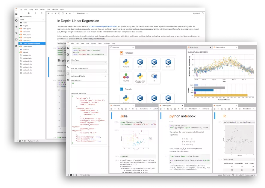
Jupyter Notebook is a web-based, open-source coding environment allowing users to write code and add well-formed notes. It can be accessed through a browser, enabling users to execute code and collaborate with other editors in real time.

Which languages does it support?

You can execute dozens of programming languages in a Jupyter Notebook with a suitable kernel. To run it, however, you need Python installed on your machine. For this article's sake, I will also limit our language to Python.

What about JupyterLab?

JupyterLab is a powerful interface that also supports Jupyter Notebook! You can go with Jupyter Notebook, but you will miss out on some neat features that JupyterLab components can offer us!

We will discuss them later. Nowadays, you have multiple choices for running your computational notebooks. You can run them on the web, or you can run them locally. The usage is similar, so it would be better to learn how to install them locally.

For better or worse, it also has multiple options. But don't be scared! The first option is the most common one. Download it from Anaconda and run JupyterLab from the Anaconda Navigator panel. As easy as it sounds! If you have another package distributor, you can also use it!

However, that option might only be suitable for some. The installation package is large, so installing might take time.

The second option is to install it as the Python package using the old and good `pip`. It's simple, but it has some drawbacks as well. For example, since we will work with Python, we need to install all libraries we will work with manually. It gives us an advantage to try and explore the latest (7, as of now) version of the notebook! Let's get started and install JupyterLab.

Setting up the environment

Make sure that you have installed and updated Python!

Go to the menu bar and create a folder in the directory where you want to place our little science project. Write `python -m venv venv` in this folder to create a virtual environment. Activate the environment. On Windows, it can be done with `.\venv\Scripts\Activate.ps1` (if you have some issues, you might want to update `pip` and `python -m pip install --upgrade pip`).

To install JupyterLab, write `pip install JupyteLab ipywidgets` to the console.

To run JupyterLab, input `jupyter lab` to the console. The tab with the lab will be opened automatically at http://localhost:8888/lab or a similar address.

You can change some UI settings (font size, theme, etc.).

First run:

‍

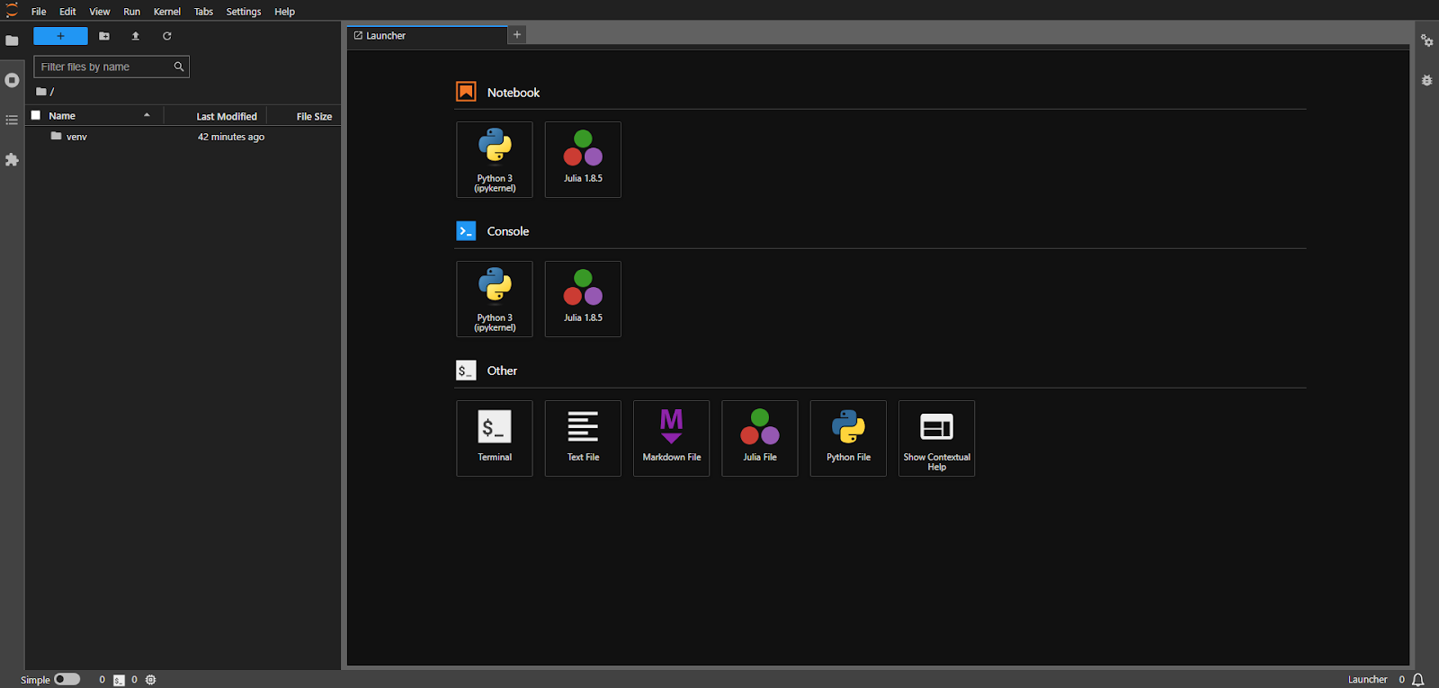
To create a notebook file, go to File -> New -> Notebook and pick `ipykernel`, or just click Python 3 (ipykernel) at the launcher tab. Rename it if necessary.

The first thing to notice is the extension— .ipynb. Note that even if it means IPython Notebook (I stands for Interactive), the programming language it can run depends on the kernel that you choose at the start.

Let's quickly go through the navigation tab:

1. Save
2. Add a cell under the current cell
3. Remove the active cell
4. Copy cells
5. Paste cell
6. Run the cell
7. Interrupt the whole kernel (not just the cell!)
8. Restart the kernel
9. Restart the kernel and run the entire list of cells
10. Choose the cell type
11. Debug mode
12. Current kernel
13. Kernel status (e.g., running or IDLE)

Demonstration of the kernel status:

‍

All these icons are very intuitive. If you want, you can learn shortcuts by pressing Help -> Show Keyboard Shortcuts.

What is a code cell?

A cell is the area where you write your code. You can write as many lines of code as necessary. Press the play button or shift + enter to execute the code.

It's not necessary to use print if the output line is the last one! In practice, people leave the variable they want to see at the end.

Here is a small demonstration:

More features

Let's examine our cells more closely! One crucial aspect is the ability to move cells around within a single notebook document and between multiple notebooks. It can significantly simplify the process of rearranging code. While the latter example may seem trivial, imagine having many images, numerous LaTeX formulas, or extensive markdown notes. Keep in mind that you should copy cells between notebooks rather than just rearranging them.

‍

Alright. Is there more on the plate? Of course! It's time to enter the magic world!

Let's start with the fact that you can use shell functions inside the Jupyter Notebook.

Just write what you want by adding `!` at the beginning. For example, write `!pip install matplotlib` and execute the cell to get the result.

To get the whole possible magic command palette, type `%lsmagic` inside the notebook! Note that when you type it, you will see the line and cell types. `line` means you need to use just %, and it acts only on one line, and `cell` means that you need to use %%, and it will act on a whole cell.

For now, we will look at just a handful of them.

%timeit

Invokes the Python's timeit module.

%hist shows the input history

If you forgot what and where you typed, and it's essential to you, use `%hist -g` to get a global history of commands (don't disclose any sensitive info 😬).

‍

%pastebin

Upload your code at https://dpaste.com. Again, don’t put your password here! 😅

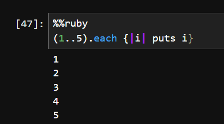
Let's look at the block magic!

‍

%%ruby

Work with Ruby if you have installed it! For example, let's count from 1 to 5. :)

%%ruby

(1..5).each {|i| puts i}

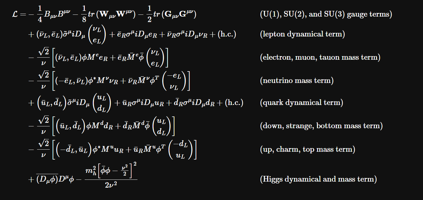
%%latex

Allows you to write latex! 

%%latex
$$
\begin{align*}
    \mathcal{L} = &-\frac{1}{4} B_{\mu\nu}B^{\mu\nu} - \frac{1}{8}\mathrm{tr}\left(\mathbf{W}_{\mu\nu}\mathbf{W}^{\mu\nu}\right) - \frac{1}{2}\mathrm{tr}\left(\mathbf{G}_{\mu\nu}\mathbf{G}^{\mu\nu}\right) && \text{(U(1), SU(2), and SU(3) gauge terms)} \\
    &+ \left(\bar{\nu}_L,\bar{e}_L\right)\tilde{\sigma}^\mu iD_\mu\begin{pmatrix}\nu_L\\e_L\end{pmatrix} + \bar{e}_R\sigma^\mu iD_\mu e_R + \bar{\nu}_R\sigma^\mu iD_\mu\nu_R + \text{(h.c.)} && \text{(lepton dynamical term)} \\
    &-\frac{\sqrt{2}}{\nu}\left[\left(\bar{\nu}_L,\bar{e}_L\right)\phi M^ee_R+\bar{e}_R\bar{M}^e\bar{\phi}\begin{pmatrix}\nu_L\\e_L\end{pmatrix}\right] && \text{(electron, muon, tauon mass term)} \\
    &-\frac{\sqrt{2}}{\nu}\left[\left(-\bar{e}_L,\bar{\nu}_L\right)\phi^{*}M^\nu\nu_R+\bar{\nu}_R\bar{M}^\nu\phi^T\begin{pmatrix}-e_L\\\nu_L\end{pmatrix}\right] && \text{(neutrino mass term)} \\
    & +\left(\bar{u}_L, \bar{d}_L\right)\tilde{\sigma}^\mu iD_\mu \begin{pmatrix}u_L\\d_L\end{pmatrix} + \bar{u}_R\sigma^\mu iD_\mu u_R + \bar{d}_R\sigma^\mu iD_\mu d_R + \text{(h.c.)} && \text{(quark dynamical term)} \\
    &- \frac{\sqrt{2}}{\nu}\left[\left(\bar{u}_L,\bar{d}_L\right)\phi M^dd_R+\bar{d}_R\bar{M}^d\bar{\phi}\begin{pmatrix}u_L\\d_L\end{pmatrix}\right] && \text{(down, strange, bottom mass term)} \\
    &-\frac{\sqrt{2}}{\nu}\left[\left(-\bar{d}_L,\bar{u}_L\right)\phi^{*}M^uu_R+\bar{u}_R\bar{M}^u\phi^T\begin{pmatrix}-d_L\\u_L\end{pmatrix}\right] && \text{(up, charm, top mass term)} \\
    &+\overline{\left(D_\mu\phi\right)}D^\mu\phi-\frac{m_h^2\left[\bar{\phi}\phi-\frac{\nu^2}{2}\right]^2}{2\nu^2} && \text{(Higgs dynamical and mass term)}
\end{align*}
$$

Fortunately, the output for latex code is more satisfying:

Let's look at HTML, SVG, and MarkDown:

‍

%%svg

https://www.python.org/static/community_logos/python-logo-generic.svg

‍

%%html

<p style="color: green; font-size: 60px;">This is nice.</p>

‍

%%markdown

### __Buy__:

- APPLE

- BLACKBERRY

- ~~INTEL~~

As you probably noticed, most notebooks don't use the %%html or %%markdown syntax.

The answer to that is simple. You can change the type of the cell to markdown and execute the cell normally. Each cell is in the `code` mode by default, making it suitable for code.

If you don't want either, choose the `Raw` to make a plain text cell.

There is plenty of unexplored magic left. You can refer to https://ipython.readthedocs.io/en/stable/interactive/magics.html#cell-magics for more info.

Collaboration on projects

Did you know that you can collaborate with others? If you don't, it's the right time to try it.

First, install the following package: `pip install jupyter-collaboration`.

After that, you can share the link with your team or friends. Be careful; you must use a reachable notebook server from the outside, not a local host.

You can also see the list of all participants on the left side.

‍

Additional features

‍

Besides the coding flow, JupyterLab has quick access to the terminal and the regular IPython console. You can create them in the same way as you created your notebook.

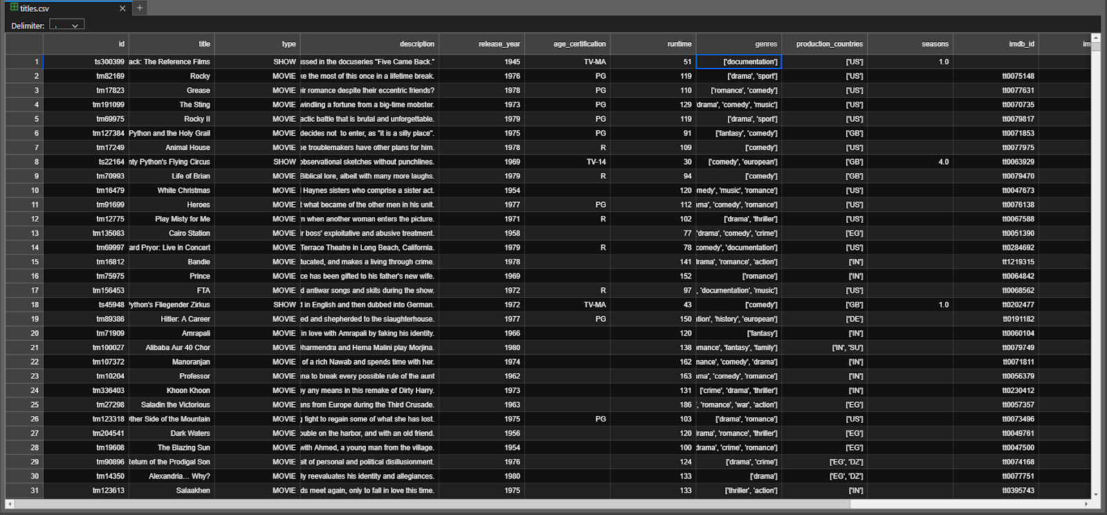
Another nice feature of JupyterLab is that it formats .csv files beautifully. It loads them fast and allows you to investigate the file quickly.

‍

Markdown files have a nice preview, no need to search for external tools. Everything is within the JupyterLab!

Fear not; Jupyter Notebook has a step-by-step debugger. Set your notebook to the debugging mode, place a breakpoint, and look for bugs.

Last but not least, the interactive plots. Write pip install plotly pandas in the terminal to process this code.

import plotly.graph_objects as go
import pandas as pd
import numpy as np
# Read data from a csv
z_data = pd.read_csv('https://raw.githubusercontent.com/plotly/datasets/master/api_docs/mt_bruno_elevation.csv')
z = z_data.values
sh_0, sh_1 = z.shape
x, y = np.linspace(0, 1, sh_0), np.linspace(0, 1, sh_1)
fig = go.Figure(data=[go.Surface(z=z, x=x, y=y)])
fig.update_layout(title='Mt Bruno Elevation', autosize=False,
                  width=500, height=500,
                  margin=dict(l=65, r=50, b=65, t=90)

Wrapping up

As you may have noticed, JupyterLab is a highly capable, resilient, and versatile computational workspace. It has the potential to streamline your tasks, enhance your efficiency, and elevate the quality of your presentations. Invest some time in familiarizing yourself with Jupyter Notebook and its functionalities. Refer to the documentation to apply your newfound knowledge to actual projects, and don't be intimidated by them any longer! Personalize your JupyterLab environment, incorporate beneficial extensions, and remember to collaborate with others and showcase your work.

‍

Related Hyperskill topics

• The Jupyter Notebook
• Installing packages with pip
• Google Colab

‍