NumPy Binomial Distribution

The binomial distribution is a probability distribution that describes the number of successes in a fixed number of independent Bernoulli trials, each with the same probability of success. It is an essential concept in probability theory and statistics, commonly used in fields such as finance, biology, and quality control. Understanding the binomial distribution allows us to predict the probability of obtaining a certain number of successes in a given number of trials, providing a foundation for more complex statistical analyses.

Importance of Binomial Distribution in Probability Theory

The binomial distribution plays a crucial role in probability theory as it models independent trials with fixed success/failure outcomes. In many real-life situations, events can be viewed as a series of independent trials, such as flipping a coin or conducting a series of medical tests. The binomial distribution helps determine the probability of a specific number of successes occurring in a fixed number of trials with a known probability of success.

For example, suppose we want to study the number of heads obtained when flipping a fair coin 10 times. Each flip of the coin can be considered an independent trial with two possible outcomes: success (heads) or failure (tails). The binomial distribution can then be used to calculate the probability of obtaining a specific number of heads, such as 5. This distribution gives us a clear understanding of the range of possible outcomes and the corresponding probabilities.

Understanding Probability Mass Function (PMF) in NumPy Binomial Distribution

Probability Mass Function (PMF) is a fundamental concept in probability theory that measures the probability of each possible outcome of a discrete random variable. In the context of the NumPy binomial distribution, the PMF provides a framework for understanding the likelihood of obtaining a certain number of successes in a fixed number of trials. By utilizing NumPy, we can generate and analyze binomial distributions and gain insight into the probabilities associated with different outcomes.

What is a Probability Mass Function?

A Probability Mass Function (PMF) is a mathematical function that provides the probability distribution for a discrete random variable. It assigns probabilities to each possible outcome of the random variable. The main components of a PMF include the random variable (representing the outcome of interest), the total number of trials, the probability of success, and the probability of failure.

The PMF of a binomial distribution is computed using the binomial coefficient, which represents the number of ways to choose a certain number of successes from a given number of trials. The formula for the binomial coefficient is:

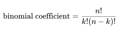
binomial coefficient=n!k!(n−k)!\text{binomial coefficient} = \frac{n!}{k!(n - k)!}binomial coefficient=k!(n−k)!n!

where nnn is the number of trials and kkk is the number of successes. The PMF is then calculated by multiplying the binomial coefficient by the probability of success raised to the power of the number of successes and the probability of failure raised to the power of the difference between the number of trials and the number of successes.

How to Calculate PMF in NumPy Binomial Distribution

To calculate the PMF in the NumPy binomial distribution, we can use the binom.pmf function from the SciPy library. This function allows us to define the values for the number of trials, probability of success, and sample size.

First, let's import the necessary libraries:

python

Copy code

import numpy as np
import scipy.stats as stats
import matplotlib.pyplot as plt

Next, we can define the parameters for the binomial distribution:

python

Copy code

n = 10 # number of trials
p = 0.5 # probability of success
size = 1000 # sample size

To calculate the PMF, we use the pmf method from the binom distribution:

python

Copy code

x = np.arange(n + 1) # possible outcomes
pmf = stats.binom.pmf(x, n, p) # calculate PMF

Finally, we can visualize the results using a bar plot:

python

Copy code

plt.bar(x, pmf)
plt.xlabel('Number of Successes')
plt.ylabel('Probability')
plt.title('Probability Mass Function of Binomial Distribution')
plt.show()

By following these steps, we can calculate the PMF in the NumPy binomial distribution and visualize it using a plot.

Examples of PMF Calculations Using NumPy

To calculate the PMF using NumPy, import the necessary libraries:

python

Copy code

import numpy as np
from scipy.stats import binom

Next, define the values for the binomial distribution:

python

Copy code

n = 10
p = 0.5
values = np.linspace(0, n, n + 1)

Calculate the PMF using the binom.pmf function:

python

Copy code

pmf = binom.pmf(values, n, p)
print(pmf)

This will display the PMF values for the specified binomial distribution.

Exploring Output Shape in NumPy Binomial Distribution

Determining the Shape of the Output Array

To determine the shape of the output array, examine the dimensions and sizes of the input arrays. The number of dimensions in the input arrays corresponds to the number of axes in the output array. Each dimension represents a specific axis along which the elements are distributed.

For example, if the input arrays have compatible dimensions and sizes, the mathematical operations will result in an output array with the same size along each axis. If the dimensions and sizes are not compatible, broadcasting may occur, where the smaller array is repeated or stretched to match the size of the larger array along certain axes.

Visualizing Output Shape with Examples

To visually represent the output shape in Python, use plotting libraries such as Matplotlib or Seaborn. For example, to visualize a histogram of a list of numbers:

python

Copy code

import matplotlib.pyplot as plt

data = [1, 2, 2, 3, 3, 3, 4, 4, 5, 5, 6, 6, 6, 7, 8]
plt.hist(data)
plt.xlabel('Value')
plt.ylabel('Frequency')
plt.show()

To visualize a scatter plot showing the relationship between two variables:

python

Copy code

import matplotlib.pyplot as plt

x = [1, 2, 3, 4, 5]
y = [2, 4, 6, 8, 10]
plt.scatter(x, y)
plt.xlabel('X')
plt.ylabel('Y')
plt.show()

Impact of Input Parameters on Output Shape

The input parameters, including size, scale, rotation, and color, significantly influence the resulting shape output. Size affects the final appearance, scale relates to the proportion of the shape to its original size, rotation determines the orientation, and color impacts the visual appeal.

For example, increasing both size and scale results in a larger and more distorted shape, while changing the rotation angle introduces a sense of movement. Altering the color scheme can transform the mood and perception of the shape.

Generating Random Samples with NumPy Binomial Distribution

Generating Random Samples Using NumPy Functions

To generate random samples using NumPy functions, utilize the numpy.random.binomial function. This function allows for the generation of random samples from a binomial distribution by specifying parameters such as the number of trials and probability of success.

For example, to generate random samples from a binomial distribution with 10 trials and a probability of success of 0.5:

python

Copy code

import numpy as np
samples = np.random.binomial(n=10, p=0.5, size=1000)

Controlling Sample Size and Seed for Reproducibility

To control sample size and seed for reproducibility, specify the desired sample size and set a seed value. The sample size determines the number of observations, while the seed value ensures consistent and reproducible randomization.

For example, to generate a sample size of 1000 and set a seed value for reproducibility:

python

Copy code

import numpy as np
np.random.seed(42)
samples = np.random.binomial(n=10, p=0.5, size=1000)

Analyzing Random Samples for Statistical Inference

Analyzing random samples for statistical inference involves selecting a random sample, determining an appropriate sample size, and conducting statistical tests. Common statistical tests include t-tests, chi-square tests, correlation analyses, and regression analyses.

For example, to analyze the random samples generated:

python

Copy code

import numpy as np
import scipy.stats as stats

n = 10
p = 0.5
samples = np.random.binomial(n, p, 1000)
mean = np.mean(samples)
std_dev = np.std(samples)

Comparing Binomial Distribution with Normal Distribution in NumPy

In NumPy, we can compare the binomial distribution and the normal distribution by examining their similarities and differences.

The binomial distribution is characterized by two parameters: n (number of trials) and p (probability of success). It models the number of successes in a fixed number of trials, each with the same probability of success. The normal distribution, also known as the Gaussian distribution, is described by its mean (μ) and standard deviation (σ). It is a continuous probability distribution that is symmetric and bell-shaped.

One similarity between the two distributions is that the binomial distribution can be approximated by the normal distribution under certain conditions. As the number of trials in the binomial distribution increases and the probability of success remains moderate, the shape of the binomial distribution becomes more bell-shaped and can be well-approximated by the normal distribution.

To generate random numbers from both distributions using NumPy:

python

Copy code

import numpy as np

# Binomial distribution
binomial_samples = np.random.binomial(n=10, p=0.5, size=1000)

# Normal distribution
normal_samples = np.random.normal(loc=0, scale=1, size=1000)

By comparing these functions and their outputs, we can further understand the similarities and differences between the binomial and normal distributions in NumPy.